Source Data

Types of Data

The current version of refine.bio is designed to process gene expression data. This includes both microarray data and RNA-seq data. We normalize data to Ensembl gene identifiers and provide abundance estimates.

More precisely, we support microarray platforms based on their GEO or ArrayExpress accessions. We currently support Affymetrix microarrays and Illumina BeadArrays, and we are continuing to evaluate and add support for more platforms. This table contains the microarray platforms that we support. We process a subset of Affymetrix platforms using the BrainArray Custom CDFs, which are denoted by a y in the is_brainarray column. We also support RNA-seq experiments performed on these short-read platforms. For more information on how data are processed, see the Processing Information section of this document. If there is a platform that you would like to see processed, please file an issue on GitHub. If you would prefer to report issues via e-mail, you can also email requests@ccdatalab.org.

Sources

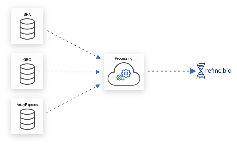
We download gene expression information and metadata from EBI’s ArrayExpress, NCBI’s Gene Expression Omnibus (GEO), and NCBI’s Sequence Read Archive (SRA). NCBI’s SRA also contains experiments from EBI’s ENA (example) and the DDBJ (example).

Metadata

We provide metadata that we obtain from the source repositories. We also attempt to, where possible, perform some harmonization of metadata to improve the discoverability of useful data. Note that we do not yet obtain sample metadata from the BioSample database, so the metadata available for RNA-seq samples is limited.

refine.bio-harmonized Metadata

The documentation in this section reflects data that has been processed via refine.bio as of version v1.45.0. See the documentation sidebar for the current version of refine.bio. The refinebio_processor_version field in the downloaded metadata file captures the refine.bio version when a sample was processed.

Scientists who upload results don’t always use the same names for related values. This makes it challenging to search across datasets. We have implemented some processes to smooth out some of these issues.

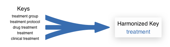
To aid in searches and for general convenience, we combine certain fields based on similar keys to produce lightly harmonized metadata. For example, treatment, treatment group, treatment protocol, drug treatment, and clinical treatment fields get collapsed down to treatment. The fields that we currently collapse to includes specimen part, genetic information, disease, disease stage, treatment, race, subject, compound, cell_line, and time.

See the table below for the mappings between the keys from source data and the harmonized keys. In addition to the source data keys explicitly listed in the table, we check for variants in the metadata from the source repositories, e.g., the source keys age, characteristic [age], and characteristic_age would all map to the harmonized key age.

Harmonized key	Keys from data sources
specimen part	organism part, cell type, tissue, tissue type, tissue source, tissue origin, source tissue, tissue subtype, tissue/cell type, tissue region, tissue compartment, tissues, tissue of origin, tissue-type, tissue harvested, cell/tissue type, tissue subregion, organ, cell_type, organismpart, isolation source, tissue sampled, cell description
genetic information	strain/background, strain, strain or line, background strain, genotype, genetic background, genotype/variation, ecotype, cultivar, strain/genotype, strain background
disease	disease , disease state , disease status , diagnosis , disease , infection with , sample type
disease stage	disease state , disease staging , disease stage , grade , tumor grade , who grade , histological grade , tumor grading , disease outcome , subject status
treatment	treatment, treatment group, treatment protocol, drug treatment, clinical treatment
race	race, ethnicity, race/ethnicity
subject	subject , subject id , subject/sample source id , subject identifier , human subject anonymized id , individual , individual identifier , individual id , patient , patient id , patient identifier , patient number , patient no , donor id , donor , sample_source_name
compound	compound, compound1, compound2, compound name, drug, drugs, immunosuppressive drugs
time	time, initial time point, start time, stop time, time point, sampling time point, sampling time, time post infection
age	age, patient age, age of patient, age (years), age at diagnosis, age at diagnosis years
cell_line	cell line
sex	sex, gender, subject gender, subject sex

Values are stripped of white space and forced to lowercase.

When multiple source keys that map to the same harmonized key are present in metadata from sources, we sort values in alphanumeric ascending order and concatenate them, separated by ;. For example, a sample with tissue: kidney and cell type: B cell would become specimen_part: B cell;kidney when harmonized.

We type-cast age values to doubles (e.g., 12 and 12 weeks both become 12.000). Because of this type-casting behavior, we do not support multiple source keys; the value harmonized to age will be the first value that is encountered. If the values can not be type-cast to doubles (e.g., “9yrs 2mos”), these are not added to the harmonized field. We do not attempt to normalize differences in units (e.g., months, years, days) for the harmonized age key. Users should consult the submitter-supplied information to determine what unit is used.

Sex is a special case; we map to female and male values if the values are one of the following:

Harmonized sex value	Values
female	f, female, woman
male	m, male, man

Only harmonized values are displayed in the sample table on the web interface. When downloading refine.bio data, these harmonized metadata are denoted with the refinebio_ prefix.

We recommend that users confirm metadata fields that are particularly important via the submitter-supplied metadata. If you find that the harmonized metadata does not accurately reflect the metadata supplied by the submitter, please file an issue on GitHub so that we can resolve it. If you would prefer to report issues via e-mail, you can also email requests@ccdatalab.org.

Submitter Supplied Metadata

We also capture the metadata as submitted to the source repositories. This includes experiment titles and descriptions or abstracts. Protocol information, which generally contains the type of sample preparation, is handled differently by different databases. We push this information down to the sample level and provide it that way. In the case of data imported from ArrayExpress, the protocol may be the information from the full experiment and not just the sample in question. Sample metadata in their original, unharmonized form are available as part of refine.bio downloads.

Processing Information

refine.bio processed

Because refine.bio is designed to be consistently updated, we use processing and normalization methods that operate on a single sample wherever possible. Processing and normalization methods that require multiple samples (e.g., Robust Multi-array Average or RMA) generally have outputs that are influenced by whatever samples are included and rerunning these methods whenever a new sample is added to the system would be impractical.

Microarray pipelines

Affymetrix

SCAN (Single Channel Array Normalization) is a normalization method for develop for single channel Affymetrix microarrays that allows us to process individual samples. SCAN models and corrects for the effect of technical bias, such as GC content, using a mixture-modeling approach. For more information about this approach, see the primary publication (Piccolo, et al. Genomics. 2012.) and the SCAN.UPC Bioconductor package documentation. We specifically use the SCANfast implementation of SCAN and the Brainarray packages as probe-summary packages when available. When available, we use BrainArray Custom CDFs during processing with SCAN.

Affymetrix platform detection

We have encountered instances where the platform label from the source repository and the metadata included in the sample’s raw data file (.CEL file) itself do not match. In these cases, we take the platform information included in the raw data (.CEL) file header to be the true platform label.

Illumina BeadArrays

Dr. Stephen Piccolo, the developer of SCAN, has adapted the algorithm for use with Illumina BeadArrays for refine.bio. Because this Illumina SCAN methodology is not yet incorporated into the SCAN.UPC package, we briefly summarize the methods below.

We require that non-normalized or raw expression values and detection p-values to be present in Illumina non-normalized data. If we infer that background correction has not occurred in the non-normalized data (e.g., there are no negative expression values), the data are background corrected using the limma::nec function (Shi, Oshlack, and Smyth. Nucleic Acids Research. 2010.). Following background correction – either upstream presumably in the Illumina BeadStudio software or in our processor, arrays are normalized with SCAN. SCAN requires probe sequence information obtained from the Illumina BeadArray Bioconductor annotation packages (e.g., illuminaHumanv1.db). We only retain probes that have a “Good” or “Perfect” rating in these packages; this quality rating is in reference to how well a probe is likely to measure its target transcript.

Illumina platform detection

We infer the Illumina BeadArray platform that a sample is likely to be run on by comparing the probe identifiers in the unprocessed file to probes for each of the Illumina expression arrays for a given organism. We again use the Illumina Bioconductor annotation packages for this step. For instance, the overlap between the probe identifiers in a human sample and the probe identifiers in each human platform (v1, v2, v3, and v4) is calculated. The platform with the highest overlap (provided it is >75%) is inferred to be the true platform. Some analyses around this platform detection procedure can be found in this repository.

Handling Illumina probes that map to multiple Ensembl gene identifiers

Illumina probes sometimes map to multiple Ensembl gene identifiers when using the annotation in Illumina BeadArray Bioconductor annotation packages (e.g., illuminaHumanv1.db). For human platforms in particular, these genes tend to be from highly polymorphic loci, e.g., Killer-cell immunoglobulin-like receptors. Because refine.bio allows users to combine samples from multiple platforms, we prioritize Ensembl gene identifiers that maximize compatibility with other platforms. Specifically, we select genes in order of priority as follows:

• Pick the gene ID with the most appearances in BrainArray packages for Affymetrix platforms of the same species as the input Illumina platform

• If two or more of the associated gene IDs appear an equal number of times in BrainArray packages, or if none of the associated gene IDs appear in any BrainArray package, we break ties as follows:

  • First, we check Ensembl and filter out any gene IDs that are no longer valid

  • Next, if there are any Ensembl genes on the primary assembly, we take only the genes on the primary assembly and discard genes in <a href”https://www.ensembl.org/info/genome/genebuild/haplotypes_patches.html” target = “blank”>haplotypes (alternative versions of the genome) or patches.

  • If there are still two or more genes left, we pick the gene with the lowest Ensembl gene identifier to break the tie. This is an arbitrary but consistent way to break ties.

This is implemented in AlexsLemonade/illumina-refinery.

RNA-seq pipelines

We use Salmon and tximport to process all RNA-seq data in refine.bio. We obtain sra files run on our supported short-read platforms from NCBI Sequence Read Archive. We use fastq-dump to named pipes, which allows us to support paired-end experiments, and pass these to Salmon. Note that any unmated reads from paired experiments are discarded.

We use the library strategy and library source metadata fields to identify RNA-seq experiments. It’s possible that experiments that are inappropriate for use with Salmon will still appear in refine.bio (e.g., long-read platforms that are labeled incorrectly in the source repository). We also encounter trouble distinguishing single-cell and bulk RNA-seq data from these fields. We strongly recommend exercising caution when using single-cell data from refine.bio as the pipeline we use may be inappropriate (e.g., correcting for gene length in 3’ tagged RNA-seq data induces bias [ref], Salmon TPM may overcorrect expression of long genes [ref]). If you find an experiment that you believe is inappropriate for use with our pipeline, please file an issue on GitHub so that we can resolve it. If you would prefer to report issues via e-mail, you can also email requests@ccdatalab.org.

Salmon

Salmon is an alignment-free method for estimating transcript abundances from RNA-seq data (Patro, et al. Nature Methods. 2017.). We use it in quasi-mapping mode, which is significantly faster than alignment-based approaches and requires us to build a Salmon transcriptome index.

Transcriptome index

We build a custom reference transcriptome (using RSEM rsem-prepare-reference) by filtering the Ensembl genomic DNA assembly to remove pseudogenes, which we expect could negatively impact the quantification of protein-coding genes. This means we’re obtaining abundance estimates for coding as well as non-coding transcripts.

Building a transcriptome index with salmon index requires us to specify a value for the parameter -k that determines the size of the k-mers used for the index. The length of a read determines what k-mer size is appropriate. Consistent with the recommendations of the authors of Salmon, we use an index build with k = 31 when quantifying samples with reads with length > 75bp. We use k = 23 for shorter read lengths.

The refine.bio processed Salmon indices are available for download. You can make use of our API like so:

https://api.refine.bio/v1/transcriptome_indices/?organism__name=<ORGANISM>&length=<LENGTH>

Where <ORGANISM> is the scientific name of the species in all caps separated by underscores and <LENGTH> is either SHORT or LONG.

To obtain the zebrafish (Danio rerio) index used for >75bp reads, use:

https://api.refine.bio/v1/transcriptome_indices/?organism__name=DANIO_RERIO&length=LONG

The download_url field will allow you to download the index.

Microbial transcriptome indices

For an individual microbial species, there are often multiple genome assemblies available. Multiple assemblies from a species often reflect that multiple strains from that species have been characterized or established as laboratory strains. We use a single genome assembly, selected by domain experts, when we generate the transcriptome index used for each microbial species. The single genome assembly is typically from a common laboratory strain. This strain’s transcriptome index is used to quantify all RNA-seq data from that species, regardless of a sample’s reported strain of origin. Quantifying using a single strain background allows us to generate compendia using a single transcriptome index, but most likely results in some loss of information for samples that do not originate from that strain.

For a list of supported microbial species and the assemblies used, please see the config/organism_strain_mapping.csv file. For more context, please also visit the original GitHub issue at AlexsLemonade/refinebio#1722.

Quantification with Salmon

When quantifying transcripts with salmon quant, we take advantage of options that allow Salmon to learn and attempt to correct for certain biases in sequencing data. We include the flags --seqBias to correct for random hexamer priming and, if this is a paired-end experiment, --gcBias to correct for GC content when running salmon quant. We set the library type parameter such that Salmon will infer the sequencing library type automatically for the reads it is quantifying (-l A).

tximport

Salmon quantification is at the transcript-level. To better integrate with the microarray data contained in refine.bio, we summarize the transcript-level information to the gene-level with tximport (Soneson, Love, and Robinson. F1000 Research. 2015.).

Our tximport implementation generates “lengthScaledTPM”, which are gene-level count-scale values that are generated by scaling TPM using the average transcript length across samples and the library size. Note that tximport is applied at the experiment-level rather than to single samples. For additional information, see the tximport Bioconductor page , the tximport tutorial Importing transcript abundance datasets with tximport, and Soneson, Love, and Robinson. F1000Research. 2015..

In some cases, all samples in an experiment can not be processing using Salmon (e.g., the file available for one sample is malformed). When experiments are >80% complete and contain more than 20 samples, we may run tximport on all available samples at the time. We’ve found the effect of running tximport “early” on the resulting values to be small under these conditions. As a result, the tximport may be run on the same example multiple times; the most recent values will be available from refine.bio.

Submitter processed

Sometimes raw data for a sample is either unavailable at the source repository or exists in a form that we can not process. For microarray platforms that we support, we obtain the submitter processed expression data and use these values in refine.bio with some modification (e.g., log2-transformation where we detect it has not been performed).

As noted above, we use Ensembl gene identifiers throughout refine.bio. Submitter processed data may use other gene (or probe) identifiers that we must convert to Ensembl gene identifiers. We describe the processes for Affymetrix and Illumina data below. Note in the case of one-to-many mappings when going from the ID used by the submitter to the Ensembl gene ID, expression values are duplicated: if a probe maps to two Ensembl gene ids, those two Ensembl gene ids will both have the probe’s expression value following conversion.

Affymetrix identifier conversion

We have created custom gene mapping files for most of the Affymetrix platforms we support. Briefly, for Brainarray supported platforms, we use the Brainarray (e.g., hgu133plus2hsensgprobe) and the platform-specific annotation package from Bioconductor (e.g., hgu133plus2.db) to generate a platform-specific mapping file that includes probe IDs, Ensembl gene IDs, gene symbols, Entrez IDs, RefSeq and Unigene identifiers. The rationale for only using probes or IDs that are accounted for in the Brainarray package is two-fold: 1) Brainarray packages are updated as we learn more about the genome and 2) it allows for these submitter processed data to be more consistent with refine.bio processed data. We support identifier conversion for a limited number of platforms that either do not have a Brainarray or Bioconductory annotation packages.

The code for deriving these mappings and more details are available at https://github.com/AlexsLemonade/identifier-refinery. If you find an issue with these mappings, please file an issue on GitHub so that we can resolve it. If you would prefer to report issues via e-mail, you can also email requests@ccdatalab.org.

Illumina identifier conversion

We support conversion from Illumina BeadArray probe IDs to Ensembl gene IDs using Bioconductor Illumina BeadArray expression packages, allowing for one-to-many mappings.

Aggregations

refine.bio allows users to aggregate their selected samples in two ways: by experiment or by species. We use the term aggregate or aggregation to refer to the process of combining individual samples to form a multi-sample gene expression matrix (see also: Downloadable Files).

• By experiment: Samples that belong to the same experiment will become a single gene expression matrix. If you have selected all samples from two experiments with 10 and 15 samples, respectively, and have chosen the by experiment option, you will receive two gene expression matrices with 10 and 15 samples, respectively.

• By species: All samples assaying the same species will be aggregated into a single gene expression matrix. If you have selected three experiments each from human and mouse and the by species option, you receive two gene expression matrices that contain all human and all mouse samples, respectively.

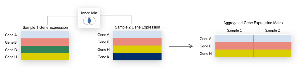
For either aggregation method, we summarize duplicate Ensembl gene IDs to the mean expression value and only include genes (rows) that are represented in all samples being aggregated. This is also known as an inner join and is illustrated below. Note that some early generation microarrays measure fewer genes than their more recent counterparts, so their inclusion when aggregating by species may result in a small number of genes being returned.

Limitations of gene identifiers when combining across platforms

We use Ensembl gene identifiers across refine.bio and, within platform, we use the same annotation to maintain consistency (e.g., all samples from the same Affymetrix platform use the same Brainarray package or identifier mapping derived from said package). However, Brainarray packages or Bioconductor annotation packages may be assembled from different genome builds compared each other or compared to the genome build used to generate transcriptome indices. If there tend to be considerable differences between (relatively) recent genome builds for your organism of interest or you are performing downstream analysis that would be sensitive to these differences, we do not recommend aggregating by species.

Transformations

Quantile normalization

refine.bio is designed to allow for the aggregation of multiple platforms and even multiple technologies. With that in mind, we would like the distributions of samples from different platforms/technologies to be as similar as possible. We use quantile normalization to accomplish this. Specifically, we generate a reference distribution for each organism from a large body of data with the normalize.quantiles.determine.target function from the preprocessCore R package and quantile normalize samples that a user selects for download with this target (using the normalize.quantiles.use.target function of preprocessCore). There is a single reference distribution per species, used to normalize all samples from that species regardless of platform or technology. We go into more detail below.

Reference distribution

By performing quantile normalization, we assume that the differences in expression values between samples arise solely from technical differences. This is not always the case; for instance, samples included in refine.bio are from multiple tissues. We’ll use as many samples as possible to generate the reference or target distribution. By including as diverse biological conditions as we have available to us to inform the reference distribution, we attempt to generate a tissue-agnostic consensus. To that end, we use the Affymetrix microarray platform with the largest number of samples for a given organism (e.g., hgu133plus2 in humans) and only samples we have processed from raw as shown below.

Quantile normalizing your own data with refine.bio reference distribution

refine.bio quantile normalization reference distribution or “targets” are available for download. You may wish to use these to normalize your own data to make it more comparable to data you obtain from refine.bio.

Quantile normalization targets can be obtained by first querying the API like so:

https://api.refine.bio/v1/qn_targets/<ORGANISM>

Where <ORGANISM> is the scientific name of the species separated by underscores.

To obtain the zebrafish (Danio rerio) reference distribution, use:

https://api.refine.bio/v1/qn_targets/danio_rerio

The s3_url field will allow you to download the index.

Quantile normalizing samples for delivery

Once we have a reference/target distribution for a given organism, we use it to quantile normalize any samples that a user has selected for download. This quantile normalization step takes place after the summarization and inner join steps described above and illustrated below.

As a result of the quantile normalization shown above, Sample 1 now has the same underlying distribution as the reference for that organism.

Note that only gene expression matrices that we are able to successfully quantile normalize will be available for download.

Limitations of quantile normalization across platforms with many zeroes

Quantile normalization is a strategy that can address many technical effects, generally at the cost of retaining certain sources of biological variability. We use a single reference distribution per organism, generated from the Affymetrix microarray platform with the largest number of samples we were able to process from raw data (see Reference distribution). In cases where the unnormalized data contains many ties within samples (and the ties are different between samples) the transformation can produce outputs with somewhat different distributions. This situation arises most often when RNA-seq data and microarray data are combined into a single dataset or matrix. To confirm that we have quantile normalized data correctly before returning results to the user, we evaluate the top half of expression values and confirm that a KS test produces a non-significant p-value. Users who seek to analyze RNA-seq and microarray data together should be aware that the low-expressing genes may not be comparable across the sets.

Skipping quantile normalization for RNA-seq experiments

When selecting RNA-seq samples for download and to aggregate by experiment, users have the option to skip quantile normalization by first selecting Advanced Options and checking the “Skip quantile normalization for RNA-seq samples” box. In this case, the output of tximport will be delivered in TSV files (see our section on RNA-seq data processing with tximport). These data can be used for differential expression analysis as “bias corrected counts without an offset” as described in the Use with downstream Bioconductor DGE packages section of tximport vignette. Note that these data will be less comparable to other datasets from refine.bio because this step has been skipped.

Gene transformations

In some cases, it may be useful to row-normalize or transform the gene expression values in a matrix (e.g., following aggregation and quantile normalization). We offer the following options for transformations:

• None: No row-wise transformation is performed.

• Z-score: Row values are z-scored using the StandardScaler from scikit-learn. This transformation is useful for examining samples’ gene expression values relative to the rest of the samples in the expression matrix (either all selected samples from that species when aggregating by species or all selected samples in an experiment when aggregating by experiment). If a sample has a positive value for a gene, that gene is more highly expressed in that sample compared to the mean of all samples; if that value is negative, that gene is less expressed compared to the population. It assumes that the data are normally distributed.

• Zero to one: Rows are scaled to values [0,1] using the MinMaxScaler from scikit-learn. We expect this transformation to be most useful for certain machine learning applications (e.g., those using cross-entropy as a loss function).

In the plot below, we demonstrate the effect of different scaling options on gene expression values (using a randomly selected human dataset, microarray platform, and gene):

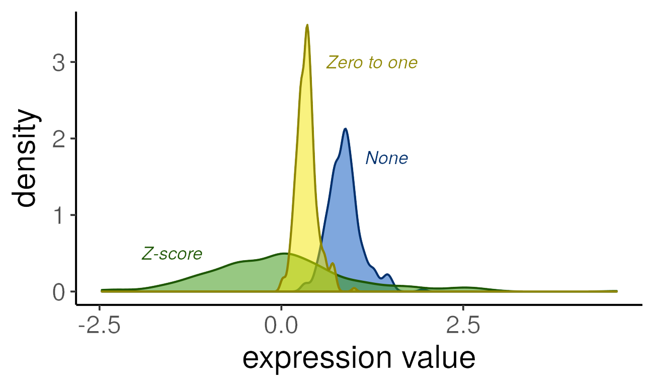
Note that the distributions retain the same general shape, but the range of values and the density are altered by the transformations.

Downloadable Files

Users can download gene expression data and associated sample and experiment metadata from refine.bio. These files are delivered as a zip file. The folder structure within the zip file is determined by whether a user selected to aggregate by experiment or by species.

The download folder structure for data aggregated by experiment:

In this example, two experiments were selected. There will be as many folders as there are selected experiments.

The download folder structure for data aggregated by species:

In this example, samples from two species were selected. There will be as many folders as there are selected experiments and this will be the case regardless of how many individual experiments were included.

In both cases, aggregated_metadata.json contains metadata, including both experiment metadata (e.g., experiment description and title) and sample metadata for everything included in the download. Below we describe the files included in the delivered zip file.

Gene Expression Matrix

Gene expression matrices are delived in tab-separated value (TSV) format. In these matrices, rows are genes or features and columns are samples. Note that this format is consistent with the input expected by many programs specifically designed for working with gene expression matrices, but some machine learning libraries will expect this to be transposed. The column names or header will contain values corresponding to sample accessions (denoted refinebio_accession_code in metadata files). You can use these values in the header to map between a sample’s gene expression data and its metadata (e.g., disease label or age). See also Downstream Analysis with refine.bio Examples.

Sample Metadata

Sample metadata is delivered in the metadata_<experiment-accession-id>.tsv, metadata_<species>.json, metadata_<species>.tsv, and aggregated_metadata.json files.

The primary way we identify samples is by using the sample accession, denoted by refinebio_accession_code. Harmonized metadata fields (see the section on harmonized metadata) are noted with a refinebio_ prefix. The refinebio_source_archive_url and refinebio_source_database fields indicate where the sample was obtained from. If there are no keys from the source data associated with a harmonized key, the harmonized metadata field will be empty. We also deliver submitter-supplied data; see below for more details. We recommend that users confirm metadata fields that are particularly important via the submitter-supplied metadata. If you find that refine.bio metadata does not accurately reflect the metadata supplied by the submitter, please file an issue on GitHub so that we can resolve it. If you would prefer to report issues via e-mail, you can also email requests@ccdatalab.org.

TSV files

In metadata TSV files, samples are represented as rows. The first column contains the refinebio_accession_code field, which match the header/column names in the gene expression matrix, followed by refine.bio-harmonized fields (e.g., refinebio_), and finally submitter-supplied values. Some information from source repositories comes in the form of nested values, which we attempt to “flatten” where possible. Note that some information from source repositories is redundant–ArrayExpress samples often have the same information in characteristic and variable fields–and we assume that if a field appears in both, the values are identical. For samples run on Illumina BeadArray platforms, information about what platform we detected and the metrics used to make that determination will also be included.

Columns in these files will often have missing values, as not all fields will be available for every sample included in a file. This will be particularly evident when aggregating by experiments that have different submitter-supplied information associated with them (e.g., one experiment contains a imatinib key and all others do not).

JSON files

Submitter supplied metadata and source urls are delivered in refinebio_annotations. As described above, harmonized values are noted with a refinebio_ prefix.

Experiment Metadata

Experiment metadata (e.g., experiment description and title) is delivered in the metadata_<species>.json and aggregated_metadata.json files.

The aggregated_metadata.json file contains additional information regarding the processing of your dataset. Specifically, the aggregate_by and scale_by fields note how the samples are grouped into gene expression matrices and how the gene expression data values were transformed, respectively. The quantile_normalized fields notes whether or not quantile normalization was performed. Currently, we only support skipping quantile normalization for RNA-seq experiments when aggregating by experiment on the web interface.

refine.bio Compendia

We periodically release compendia comprised of all the samples from a species that we were able to process. We refer to these as refine.bio compendia. We offer two kinds of refine.bio compendia: normalized compendia and RNA-seq sample compendia.

Normalized compendia

refine.bio normalized compendia are comprised of all the samples from a species that we were able to process, aggregate, and normalize. Normalized compendia provide a snapshot of the most complete collection of gene expression that refine.bio can produce for each supported organism. We process these compendia in a manner that is different from the options that are available via the web user interface. Note that submitter processed samples that are available through the web user interface are omitted from normalized compendia because these samples can introduce unwanted technical variation.

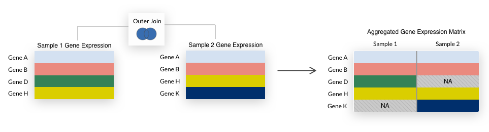
The refine.bio web interface does an inner join when datasets are combined, so only genes present in all datasets are included in the final matrix. For compendia, we take the union of all genes, filling in any missing values with NA. This is a “full outer join” as illustrated below. We use a full outer join because it allows us to retain more genes in a compendium and we impute missing values during compendia creation.

We perform an outer join each time samples are combined in the process of building normalized compendia.

Samples from each technology—microarray and RNA-seq—are combined separately. In RNA-seq samples, we filter out genes with low total counts and then log2(x + 1) the data. We join samples from both technologies. We then drop genes that have missing values in greater than 30% of samples. Finally, we drop samples that have missing values in greater than 50% of genes. We impute the remaining missing values with IterativeSVD from fancyimpute. We then quantile normalize all samples as described above.

We’ve made our analyses underlying processing choices and exploring test compendia available at our compendium-processing repository.

Collapsing by genus

Microarray platforms are generally designed to assay samples from a specific species. In some cases, publicly available data surveyed by refine.bio may include samples where the microarray platform used was not specifically designed for the species as described (e.g., samples labeled Bos indicus were run on Bos taurus microarrays or mouse crosses that are not labeled Mus musculus were run on Mus musculus microarrays). When we encounter this in refine.bio, we will include samples in a compendium from species that differ from the primary platform species when the two species share a genus (e.g., Bos indicus samples run on Bos taurus microarrays are included in the Bos taurus normalized compendium, and Mus crosses are included in the Mus musculus normalized compendium). Such non-primary species samples generally account for a small fraction of the total samples included in a normalized compendium. If you would like to filter a normalized compendium based on a sample’s species label, you can use the refinebio_organism column in the metadata TSV file or the .samples[].refinebio_organism field in the metadata JSON file included as part of the download.

Note that non-primary species samples from species that are outside the genus of the primary platform species are not currently available in any normalized compendium (e.g., Pan troglodytes samples assayed on Homo sapiens microarrays are not included in the Pan troglodytes or Homo sapiens compendia), but can be included in datasets from refine.bio.

Below is the list of organisms and their primary organisms:

Primary Organism	Organisms included in compendium
Anopheles gambiae	Anopheles gambiae
Arabidopsis thaliana	Arabidopsis thaliana, Arabidopsis halleri, Arabidopsis thaliana x arabidopsis halleri subsp. gemmifera, Arabidopsis lyrata subsp. petraea, Arabidopsis lyrata subsp. lyrata, Arabidopsis thaliana x arabidopsis lyrata, Arabidopsis halleri subsp. gemmifera, Arabidopsis lyrata
Bos indicus	Bos indicus
Bos taurus	Bos taurus, Bos indicus, Bos grunniens
Caenorhabditis elegans	Caenorhabditis elegans
Citrus sinensis	Citrus x paradisi, Citrus reticulata, Citrus sinensis, Citrus limon, Citrus reticulata x citrus trifoliata, Citrus clementina, Citrus unshiu, Citrus x tangelo, Citrus maxima
Danio rerio	Danio rerio
Drosophila melanogaster	Drosophila melanogaster, Drosophila simulans, Drosophila mauritiana, Drosophila sechellia, Drosophila teissieri, Drosophila santomea, Drosophila yakuba
Escherichia coli	Escherichia coli, Escherichia coli str. k-12 substr. mg1655, Escherichia coli k-12, Escherichia coli cft073, Escherichia coli str. k-12 substr. w3110, Escherichia coli uti89, Escherichia coli b str. rel606, Escherichia coli o157, Escherichia coli 8624, Escherichia coli sci-07, Escherichia coli bw25113, Escherichia coli apec o2, Escherichia coli str. k-12 substr. mc4100, Escherichia coli o08, Escherichia coli str. k-12 substr. dh10b
Escherichia coli k-12	Escherichia coli k-12
Escherichia coli str. k-12 substr. mg1655	Escherichia coli str. k-12 substr. mg1655
Gallus gallus	Gallus gallus
Glycine max	Glycine max, Glycine soja
Gossypium hirsutum	Gossypium herbaceum, Gossypium hirsutum, Gossypium barbadense, Gossypium arboreum
Homo sapiens	Homo sapiens
Hordeum vulgare	Hordeum vulgare, Hordeum vulgare subsp. spontaneum
Lepidium sativum	Lepidium sativum
Macaca fascicularis	Macaca fascicularis
Macaca mulatta	Macaca mulatta
Musculus	Musculus
Mus musculus	Mus musculus, Mus spretus, Mus caroli, Mus musculus musculus x m. m. domesticus, Mus musculus domesticus, Mus musculus x mus spretus, Mus musculus musculus x m. m. castaneus, Mus musculus musculus, Mus musculus castaneus, Mus sp.
Mustela putorius furo	Mustela putorius furo
Oryza sativa	Oryza sativa japonica, Oryza sativa, Oryza sativa indica group, Oryza longistaminata
Oryza sativa indica group	Oryza sativa indica group
Plasmodium falciparum	Plasmodium falciparum 3d7, Plasmodium falciparum
Populus tremula x populus alba	Populus tremula x populus alba
Populus trichocarpa	Populus trichocarpa
Populus x canadensis	Populus x canadensis
Pseudomonas aeruginosa	Pseudomonas aeruginosa, Pseudomonas aeruginosa pao1, Pseudomonas putida, Pseudomonas aeruginosa ucbpp-pa14, Pseudomonas aeruginosa pa14, Pseudomonas aeruginosa tbcf10839, Pseudomonas aeruginosa pahm4
Pseudomonas aeruginosa pao1	Pseudomonas aeruginosa pao1
Rattus norvegicus	Rattus norvegicus, Rattus rattus, Rattus norvegicus albus
Saccharomyces cerevisiae	Saccharomyces cerevisiae, Saccharomyces cerevisiae s288c, Saccharomyces pastorianus, Saccharomyces pastorianus weihenstephan 34/70, Saccharomyces cerevisiae vin13, Saccharomyces uvarum, Saccharomyces cerevisiae ec1118, Saccharomyces cerevisiae cen.pk113-7d, Saccharomyces cerevisiae by4741, Saccharomyces cerevisiae sk1, Saccharomyces bayanus, Saccharomyces cerevisiae x saccharomyces kudriavzevii, Saccharomyces boulardii
Schizosaccharomyces pombe	Schizosaccharomyces pombe, Schizosaccharomyces pombe 972h-
Staphylococcus aureus	Staphylococcus aureus, Staphylococcus aureus subsp. aureus rn4220, Staphylococcus aureus subsp. aureus n315, Staphylococcus aureus subsp. aureus usa300, Staphylococcus aureus subsp. aureus mu50, Staphylococcus aureus subsp. aureus str. newman
Sus scrofa	Sus scrofa domesticus, Sus scrofa
Triticum aestivum	Triticum aestivum, Triticum turgidum subsp. dicoccoides, Triticum turgidum subsp. durum, Triticum turgidum, Triticum carthlicum, Triticum monococcum
Vitis hybrid cultivar	Vitis hybrid cultivar
Vitis riparia	Vitis riparia
Vitis vinifera	Vitis vinifera, Vitis rotundifolia, Vitis hybrid cultivar, Vitis aestivalis, Vitis riparia, Vitis cinerea var. helleri x vitis vinifera, Vitis cinerea var. helleri x vitis rupestris, Vitis cinerea var. helleri x vitis riparia
Xenopus laevis	Xenopus muelleri, Xenopus laevis x xenopus muelleri, Xenopus laevis, Xenopus laevis x xenopus borealis, Xenopus borealis
Zea mays	Zea mays

Normalized Compendium Download Folder

Users will receive a zipped folder with a gene expression matrix aggregated by species, along with associated metadata. Below is the detailed folder structure:

RNA-Seq Sample Compendia

refine.bio RNA-seq sample compendia are comprised of the Salmon output for the collection of RNA-seq samples from an organism that we have processed with refine.bio. Each individual sample has its own quant.sf file; the samples have not been aggregated and normalized. RNA-seq sample compendia are designed to allow users that are comfortable handling these files to generate output that is most useful for their downstream applications. Please see the Salmon documentation on the quant.sf output format for more information.

RNA-Seq Sample Compendium Download Folder

Users will receive a zipped folder with individual quant.sf files for each sample that we were able to process with Salmon, grouped into folders based on the experiment those samples come from, along with any associated metadata in refine.bio. Please note that our RNA-seq sample metadata is limited at this time and in some cases, we could not successfully run Salmon on every sample within an experiment (e.g., our processing infrastructure encountered an error with the sample, the sequencing files were malformed). In addition, we use the terms “sample” and “experiment” to be consistent with the rest of refine.bio, but files will use run identifiers (e.g., SRR, ERR, DRR) and project identifiers (e.g., SRP, ERP, DRP), respectively. Below is the detailed folder structure:

API

You can use the refine.bio API to build your own applications utilizing the refine.bio processed data. You can also select samples for aggregation and download via the API with additional options for download (e.g., without quantile normalization, selecting sample-specific quant.sf files). Our quantile normalization targets and transcriptome indices are available only via the API (see Quantile normalizing your own data with refine.bio reference distribution and Transcriptome index, respectively).

For more information see our API documentation at api.refine.bio.

Downstream Analysis with refine.bio Examples

Our refine.bio examples site includes a number of different analyses you can perform with data from refine.bio in the R programming language. You can view our examples in your browser or download the R Markdown (.Rmd) files to run the code locally (find more information on required software here and how to use .Rmd here). Example analyses are designed to guide you through obtaining data from the refine.bio web interface and provide instruction for adapting the analysis for a dataset of your choice. View our Getting Started page, Introduction to Microarray, or Introduction to RNA-seq to start using refine.bio examples.

Here’s a sneak peek of examples that are available:

• Differential gene expression analysis for several groups (Microarray)

• Differential gene expression analysis for 2 groups (RNA-seq)

• Hierarchical clustering and heatmap creation (RNA-seq)

• Gene Set Enrichment Analysis (Microarray)

• Visualization with Uniform Manifold Approximation and Projection (RNA-seq)

Give us feedback on our refine.bio examples! If you have a question about or find a problem with one of our examples and need to get in touch with one of our staff, please file a GitHub issue. If you would prefer to report issues via e-mail, you can also email requests@ccdatalab.org.